How to Make a Budget Spreadsheet in Excel

Step 1: Open Excel

 

1. Begin by opening Microsoft Excel on your computer. If you don’t have Excel, you can use Google Sheets, which offers similar functionality and is available for free with a Google account.

 

Step 2: Create a New Workbook

 

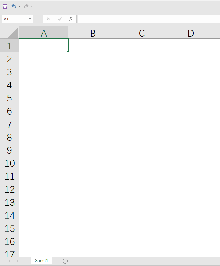
1. After launching Excel, you’ll see a blank workbook. Each workbook can contain multiple worksheets. By default, you have one worksheet called “Sheet1.”

Step 3: Rename the Worksheet

 

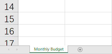
1. Double-click on the “Sheet1” tab at the bottom of the Excel window to rename it to something like “Monthly Budget.” This helps you stay organized if you plan to have multiple sheets in the same workbook.

Step 4: Set Up Your Spreadsheet

 

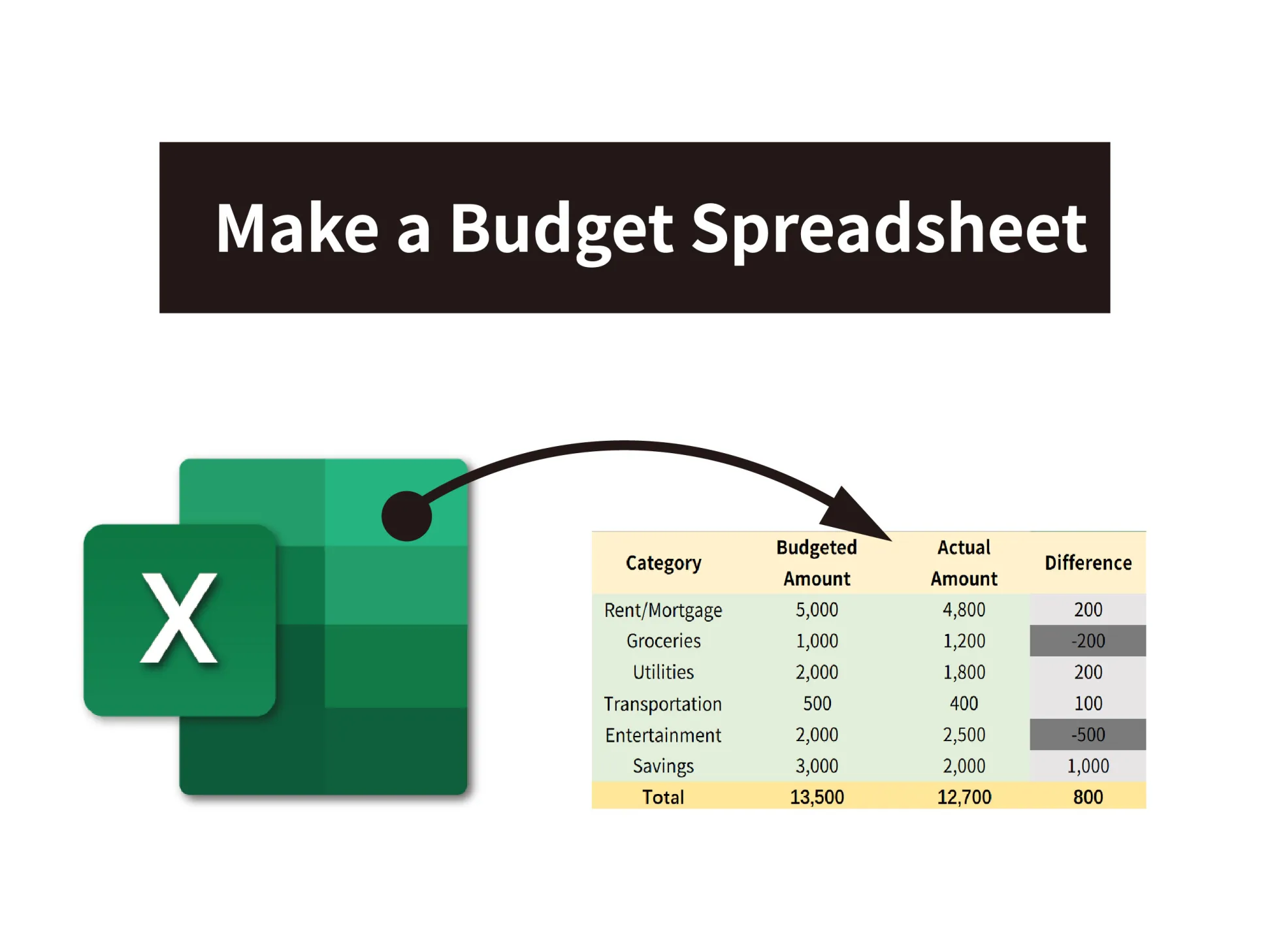
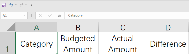
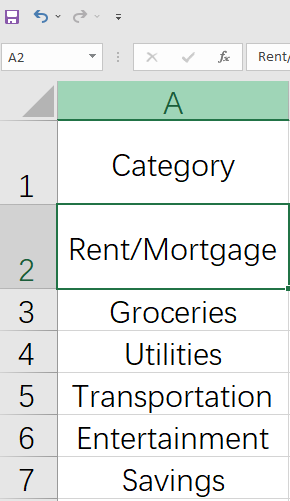
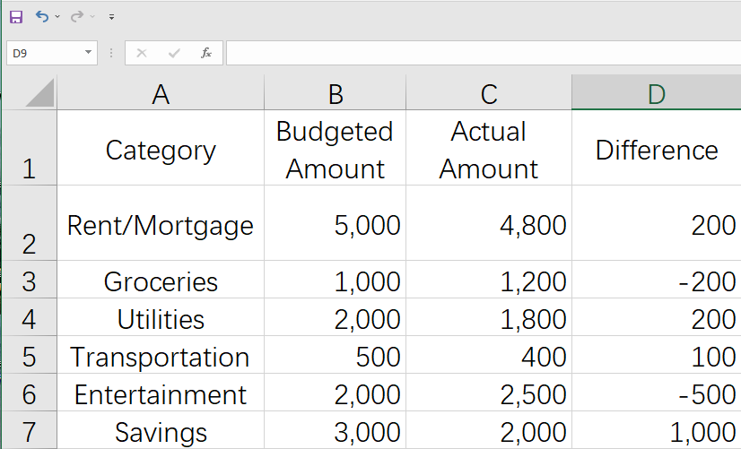
1. Label your columns. In cell A1, type “Category.” This column will list your budget categories.
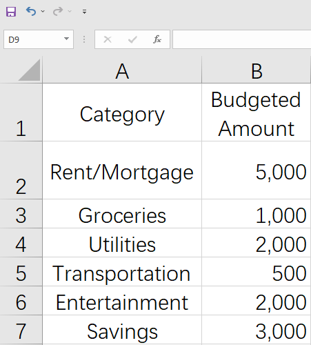
2. In cell B1, type “Budgeted Amount.” This column will contain the amount of money you plan to spend in each category.
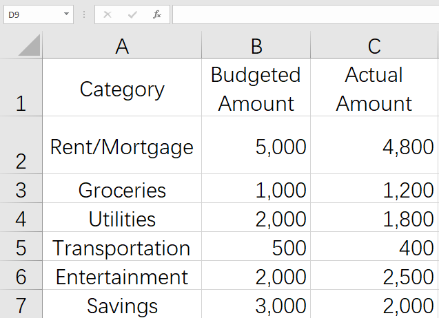
3. In cell C1, type “Actual Amount.” This column will track how much you actually spend in each category.
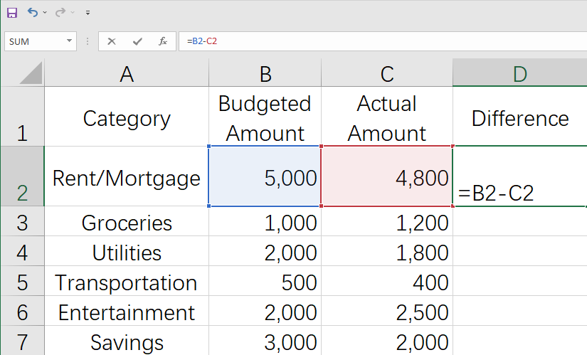
4. In cell D1, type “Difference.” This column will automatically calculate the variance between your budgeted and actual amounts.

Step 5: Enter Budget Categories

 

1. Starting from cell A2, list all your budget categories in column A (e.g., Rent/Mortgage, Groceries, Utilities, Transportation, Entertainment, Savings, etc.). You can add or remove categories as needed.

Step 6: Enter Budgeted Amounts

 

1. In column B, starting from cell B2, enter the amount of money you plan to allocate to each category for the month. These are your budgeted amounts.

Step 7: Enter Actual Expenses

 

1. In column C, starting from cell C2, enter your actual expenses for each category as you spend money throughout the month. Update these amounts whenever you make a purchase.

Step 8: Calculate the Difference

 

1. In cell D2, enter the formula `=B2-C2`. This formula calculates the difference between your budgeted amount and your actual spending for the first category.
2. Copy this formula down to apply it to all rows in column D, so it calculates the differences for all categories.

Step 9: Format Your Spreadsheet

 

1. Format your spreadsheet to make it visually appealing and easy to read. You can adjust fonts, colors, cell borders, and alignment.
2. Consider using cell shading or conditional formatting to highlight positive or negative differences, making it easier to spot areas where you’ve overspent or saved money.

Step 10: Add Total Rows

 

1. At the bottom of your category list, add a row for totals.
2. In cell A (last row + 1), type “Total.”
3. In cell B (last row + 1), enter the formula `=SUM(B2:B[last row])` to calculate the total budgeted amount.
4. In cell C (last row + 1), enter the formula `=SUM(C2:C[last row])` to calculate the total actual amount.
5. In cell D (last row + 1), enter the formula `=B[last row+1]-C[last row+1]` to calculate the overall budget difference.

 

Step 11: Use Excel Functions

 

1. Excel offers various functions to analyze your budget, such as SUM, AVERAGE, MIN, MAX, etc. You can use these functions to gain insights into your spending patterns.

 

Step 12: Regularly Update Your Spreadsheet

 

1. To keep your budget accurate, update the “Actual Amount” column as you make purchases or have changes in your budget. This will ensure you have real-time information on your finances.

 

Step 13: Save Your Spreadsheet

 

1. Click on “File” and choose “Save As” to save your budget spreadsheet with a descriptive name in a location of your choice.

 

Step 14: Review and Adjust

 

1. Periodically review your budget spreadsheet to assess your financial progress. Adjust your budgeted amounts as needed to meet your financial goals.

 

By following these detailed steps, you can create an effective budget spreadsheet in Excel to manage your finances comprehensively. Remember that budgeting is an ongoing process, and regularly updating your spreadsheet is key to financial success.